What is Numpy?
NumPy is an incredibly powerful module and a foundation of scientific computing in Python. It provides a high-performance multidimensional array object, and tools for working with these arrays.
# Import the numpy module and assign the alias np
import numpy as np
What is an array?
A numpy array is a grid of values, all of the same type, and is indexed by a tuple of nonnegative integers. The number of dimensions is the rank of the array; the shape of an array is a tuple of integers giving the size of the array along each dimension.
We can initialize numpy arrays from nested Python lists, and access elements using square brackets. Here we generate rank 1 array, a, with elements 1,2,3. Think of it as nothing more than a list with built-in methods.
a = np.array([1, 2, 3])
print(type(a))
print(a.shape)
print(a[0], a[1], a[2])
a[0] = 5
print(a)
<class 'numpy.ndarray'>
(3,)
1 2 3
[5 2 3]
? a
[0;31mType:[0m ndarray
[0;31mString form:[0m [5 2 3]
[0;31mLength:[0m 3
[0;31mFile:[0m ~/miniconda3/envs/datasci/lib/python3.7/site-packages/numpy/__init__.py
[0;31mDocstring:[0m <no docstring>
[0;31mClass docstring:[0m
ndarray(shape, dtype=float, buffer=None, offset=0,
strides=None, order=None)
An array object represents a multidimensional, homogeneous array
of fixed-size items. An associated data-type object describes the
format of each element in the array (its byte-order, how many bytes it
occupies in memory, whether it is an integer, a floating point number,
or something else, etc.)
Arrays should be constructed using `array`, `zeros` or `empty` (refer
to the See Also section below). The parameters given here refer to
a low-level method (`ndarray(...)`) for instantiating an array.
For more information, refer to the `numpy` module and examine the
methods and attributes of an array.
Parameters
----------
(for the __new__ method; see Notes below)
shape : tuple of ints
Shape of created array.
dtype : data-type, optional
Any object that can be interpreted as a numpy data type.
buffer : object exposing buffer interface, optional
Used to fill the array with data.
offset : int, optional
Offset of array data in buffer.
strides : tuple of ints, optional
Strides of data in memory.
order : {'C', 'F'}, optional
Row-major (C-style) or column-major (Fortran-style) order.
Attributes
----------
T : ndarray
Transpose of the array.
data : buffer
The array's elements, in memory.
dtype : dtype object
Describes the format of the elements in the array.
flags : dict
Dictionary containing information related to memory use, e.g.,
'C_CONTIGUOUS', 'OWNDATA', 'WRITEABLE', etc.
flat : numpy.flatiter object
Flattened version of the array as an iterator. The iterator
allows assignments, e.g., ``x.flat = 3`` (See `ndarray.flat` for
assignment examples; TODO).
imag : ndarray
Imaginary part of the array.
real : ndarray
Real part of the array.
size : int
Number of elements in the array.
itemsize : int
The memory use of each array element in bytes.
nbytes : int
The total number of bytes required to store the array data,
i.e., ``itemsize * size``.
ndim : int
The array's number of dimensions.
shape : tuple of ints
Shape of the array.
strides : tuple of ints
The step-size required to move from one element to the next in
memory. For example, a contiguous ``(3, 4)`` array of type
``int16`` in C-order has strides ``(8, 2)``. This implies that
to move from element to element in memory requires jumps of 2 bytes.
To move from row-to-row, one needs to jump 8 bytes at a time
(``2 * 4``).
ctypes : ctypes object
Class containing properties of the array needed for interaction
with ctypes.
base : ndarray
If the array is a view into another array, that array is its `base`
(unless that array is also a view). The `base` array is where the
array data is actually stored.
See Also
--------
array : Construct an array.
zeros : Create an array, each element of which is zero.
empty : Create an array, but leave its allocated memory unchanged (i.e.,
it contains "garbage").
dtype : Create a data-type.
Notes
-----
There are two modes of creating an array using ``__new__``:
1. If `buffer` is None, then only `shape`, `dtype`, and `order`
are used.
2. If `buffer` is an object exposing the buffer interface, then
all keywords are interpreted.
No ``__init__`` method is needed because the array is fully initialized
after the ``__new__`` method.
Examples
--------
These examples illustrate the low-level `ndarray` constructor. Refer
to the `See Also` section above for easier ways of constructing an
ndarray.
First mode, `buffer` is None:
>>> np.ndarray(shape=(2,2), dtype=float, order='F')
array([[ -1.13698227e+002, 4.25087011e-303],
[ 2.88528414e-306, 3.27025015e-309]]) #random
Second mode:
>>> np.ndarray((2,), buffer=np.array([1,2,3]),
... offset=np.int_().itemsize,
... dtype=int) # offset = 1*itemsize, i.e. skip first element
array([2, 3])
What if we want to extend this to a higher dimension? It’s easy! Let us create a 2x3 dimensional array.
b = np.array([[1,2,3],[4,5,6]])
print(b)
print(b.shape)
print(b[0, 0], b[0, 1], b[1, 0])
[[1 2 3]
 [4 5 6]]
(2, 3)
1 2 4
More on Array Indexing and Slicing
A powerful feature of arrays (and lists) is array indexing and slicing, which allows us to access individual elements, or subsets, of an array.
b = np.array([[1,2,3],[4,5,6]])
print(b[0]) # first row
print(b[0,0]) # first entry of the first row
print(b[0, 1:]) #first row, entries after "1"th position
print(b[1, 1:-1]) #second row, "1"th element to the penultimate.
[1 2 3]
1
[2 3]
[5]
Boolean Indexing
Boolean array indexing lets you pick out arbitrary elements of an array. Frequently this type of indexing is used to select the elements of an array that satisfy some condition. Here is an example:
print(b[b > 2]) # elements of b where are greater than 2
print(b[b != 5]) # elements of b not equal to 5
[3 4 5 6]
[1 2 3 4 6]
Exercise
1) Create the following array:
 [[ 1  2  3  4]
  [ 5  6  7  8]
  [ 9 10 11 12]]
2) Return the “Rank 1” and “Rank 2” views of the second row. Additionally, return their shapes.
3) Repeat for a column of your choice.
Exercise Solution
# (1)
a = np.array([[1,2,3,4], [5,6,7,8], [9,10,11,12]])

# (2)
row_r1 = a[1, :]
row_r2 = a[1:2, :]
print(row_r1, row_r1.shape)
print(row_r2, row_r2.shape)

# (3)
col_r1 = a[:, 1]
col_r2 = a[:, 1:2]
print(col_r1, col_r1.shape)
print(col_r2, col_r2.shape)
[5 6 7 8] (4,)
[[5 6 7 8]] (1, 4)
[ 2  6 10] (3,)
[[ 2]
 [ 6]
 [10]] (3, 1)
Creating Arrays
Numpy also provides many functions to create arrays, here are some examples:
a = np.zeros((2,2))   # Create an array of all zeros
print(a)
[[0. 0.]
 [0. 0.]]
b = np.ones((1,2))    # Create an array of all ones
print(b)
[[1. 1.]]
c = np.full((2,2), 7)  # Create a constant array
print(c)
[[7 7]
 [7 7]]
d = np.eye(2)         # Create a 2x2 "identity matrix"
print(d)
[[1. 0.]
 [0. 1.]]
f = np.arange(0, 4, 0.1)  # Create an array with elements from
                          # 0 to 4 in increments of 0.1
print(f)
[0.  0.1 0.2 0.3 0.4 0.5 0.6 0.7 0.8 0.9 1.  1.1 1.2 1.3 1.4 1.5 1.6 1.7
 1.8 1.9 2.  2.1 2.2 2.3 2.4 2.5 2.6 2.7 2.8 2.9 3.  3.1 3.2 3.3 3.4 3.5
 3.6 3.7 3.8 3.9]
g = np.linspace(0, 10, 5)  # Create an array with 5 elements
                           # between 0 and 10, linearly spaced
print(g)
[ 0. 2.5 5. 7.5 10. ]
h = np.logspace(-1, 2, 4)  # Create an array with 4 elements
                           # between 10^{-1} and 10^{2}, log spaced
print(h)
[ 0.1 1. 10. 100. ]
And lots more!
Elementwise Math on Arrays
Basic mathematical functions operate elementwise on arrays, and are available both as operator overloads and as functions in the numpy module. For example:
x = np.array([[1,2],[3,4]])
y = np.array([[5,6],[7,8]])
# Elementwise sum; both produce the array
# [[ 6.0  8.0]
#  [10.0 12.0]]
print(x + y)
print(np.add(x, y))
[[ 6  8]
 [10 12]]
[[ 6  8]
 [10 12]]
# Elementwise difference; both produce the array
# [[-4.0 -4.0]
#  [-4.0 -4.0]]
print(x - y)
print(np.subtract(x, y))
[[-4 -4]
 [-4 -4]]
[[-4 -4]
 [-4 -4]]
# Elementwise product; both produce the array
# [[ 5.0 12.0]
#  [21.0 32.0]]
print(x * y)
print(np.multiply(x, y))
[[ 5 12]
 [21 32]]
[[ 5 12]
 [21 32]]
# Elementwise division; both produce the array
# [[ 0.2         0.33333333]
#  [ 0.42857143  0.5       ]]
print(x / y)
print(np.divide(x, y))
[[0.2        0.33333333]
 [0.42857143 0.5       ]]
[[0.2        0.33333333]
 [0.42857143 0.5       ]]
# Elementwise square root; produces the array
# [[ 1.          1.41421356]
#  [ 1.73205081  2.        ]]
print(x**(1/2))
print(np.sqrt(x))
[[1.         1.41421356]
 [1.73205081 2.        ]]
[[1.         1.41421356]
 [1.73205081 2.        ]]
Matrix Math
We have just done elementwise mathematical operations, not matrix multiplication. We recognize many of you have not yet taken linear algebra, so if you are confused, please don’t be afraid to ask for help. Chances are, if you are lost, someone else is lost.
We often use an operation called a “dot product” in matrix multiplication. The dot function is used to compute the inner products of vectors–multiply a vector by a matrix–and to multiply matricies. The dot function is available as a function and an instance method.
x = np.array([[1,2],[3,4]])
y = np.array([[5,6],[7,8]])

v = np.array([9,10])
w = np.array([11, 12])
Below we compute:
\begin{equation} \begin{bmatrix} 9 & 10 \end{bmatrix} \cdot \begin{bmatrix} 11 \ 12 \end{bmatrix} = 9(11) + 10(12) = 219 \end{equation}
# Inner product of vectors; both produce 219
print(v.dot(w))
print(np.dot(v, w))
219
219
Below we compute:
\begin{equation} \begin{bmatrix} 1 & 2 \ 3 & 4 \end{bmatrix} \cdot \begin{bmatrix} 9 \ 10 \end{bmatrix} = \begin{bmatrix} 1(9) + 2(10) \ 3(9) + 4(10) \end{bmatrix} = \begin{bmatrix} 29 \ 67 \end{bmatrix} \end{equation}
# Matrix / vector product; both produce the rank 1 array [29 67]
print(x.dot(v))
print(np.dot(x, v))
[29 67]
[29 67]
Below we compute:
\begin{equation} \begin{bmatrix} 1 & 2 \ 3 & 4 \end{bmatrix} \cdot \begin{bmatrix} 5 & 6 \ 7 & 8 \end{bmatrix} = \begin{bmatrix} 19 & 22 \ 43 & 50 \end{bmatrix} \end{equation}
# Matrix / matrix product; both produce the rank 2 array
# [[19 22]
#  [43 50]]
print(x.dot(y))
print(np.dot(x, y))
[[19 22]
 [43 50]]
[[19 22]
 [43 50]]
Below we compute the “transpose” of matrix x.
\begin{equation} x^T = \begin{bmatrix} 1 & 2 \ 3 & 4 \end{bmatrix}^T = \begin{bmatrix} 1 & 3 \ 2 & 4 \end{bmatrix} \end{equation}
print(x.T) # transpose of x
[[1 3]
 [2 4]]
Exercise
1) Define a 3x3 indentity matrix, A.
2) Define a 3x3 matrix, B, with elements
 [[ 1  2  3]
  [ 4  5  6]
  [ 7 8 9]]
3) Perform the following operations:
\begin{equation} (\pi) \mathbf{A} \cdot \mathbf{B^T} + \mathbf{B} \end{equation}
Exercise Solution
# (1)
A = np.eye(3)

# (2)
B = np.arange(1,10).reshape((3,3))

# (3)
pi = np.pi
pi * np.dot(A, B.T) + B
array([[ 4.14159265, 14.56637061, 24.99114858],
       [10.28318531, 20.70796327, 31.13274123],
       [16.42477796, 26.84955592, 37.27433388]])
Numpy Random Numbers
print(np.random.random(5)) # 5 random numbers in [0,1)
[0.27670365 0.46237981 0.16295827 0.15668182 0.18904477]
print(np.random.random((3,3))) # 3x3 matrix of random numbers
[[0.73459547 0.77665021 0.60142376]
 [0.69066281 0.96342857 0.51028504]
 [0.70416279 0.13537875 0.91527968]]
print(np.random.uniform(size=5)) # 5 random numbers in [0,1]
[0.70695405 0.90766612 0.09580399 0.07638609 0.8874512 ]
print(np.random.randint(3, 10, 4)) # 4 integers between 3 and 10
[9 8 4 9]
And there are a lot of other options, see the Numpy.random documentation.
Some Basic Plotting
Here we introduce some basic forms of plotting. We will go further in depth later, but take this a template to understand the following sections. We will be using the Python library called matplotlib which introduces many powerful plotting tools.
# Import the pyplot submodule and assign the alias plt
import matplotlib.pyplot as plt
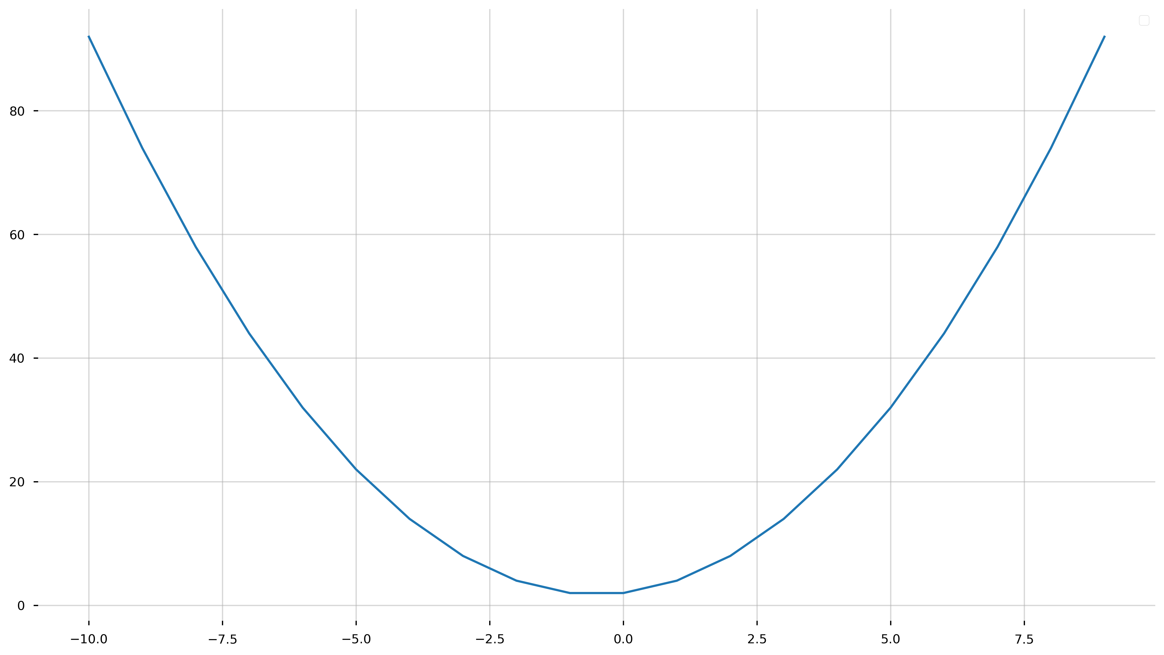
Line Plot
fig = plt.figure(figsize=(16,9))
ax = plt.gca()

x = np.arange(-10, 10, 1)
y = x**2 + x + 2.0

ax.plot(x, y)
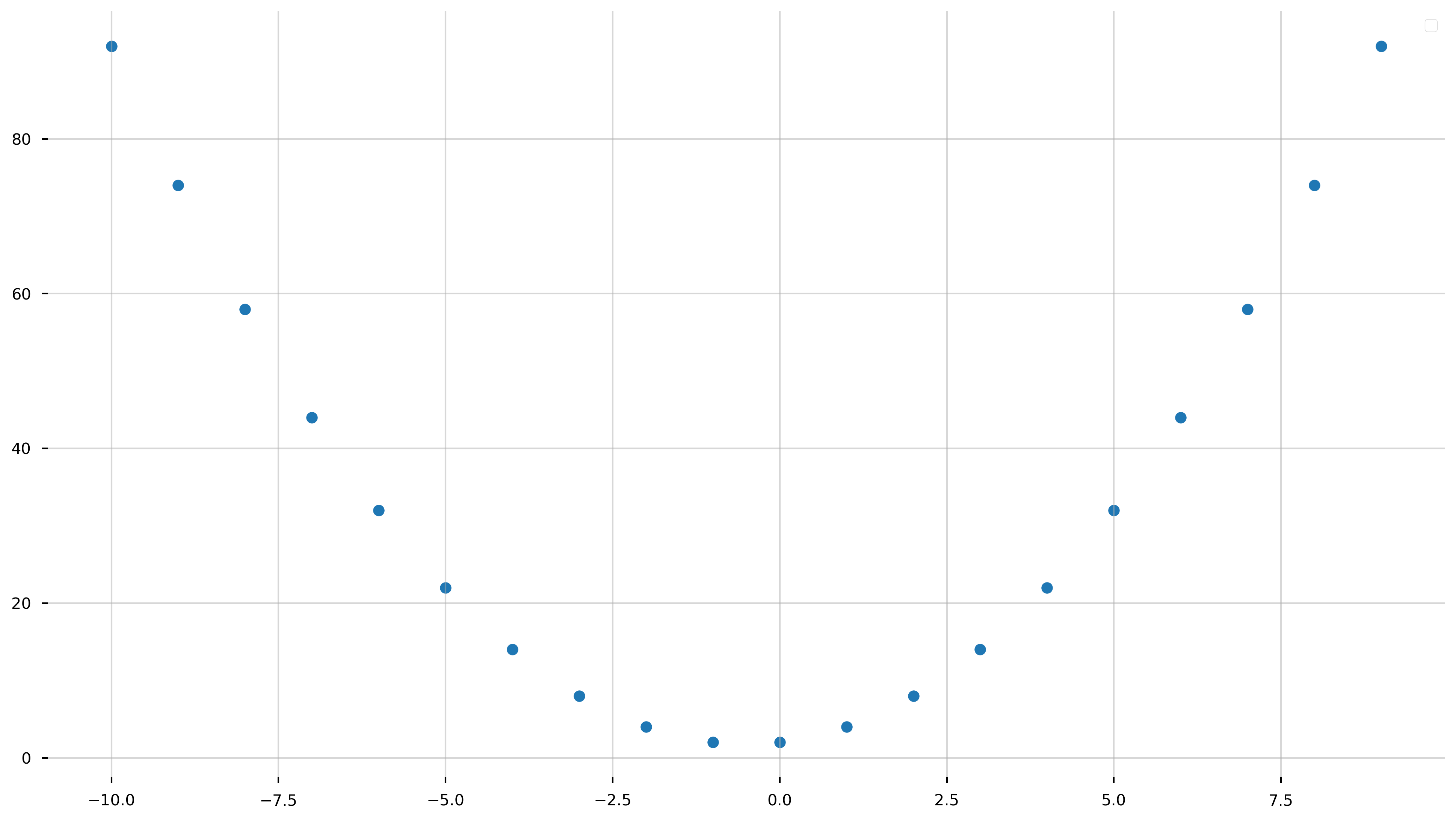
Scatter Plot
fig = plt.figure(figsize=(16,9))
ax = plt.gca()

x = np.arange(-10, 10, 1)
y = x**2 + x + 2.0

ax.scatter(x, y)
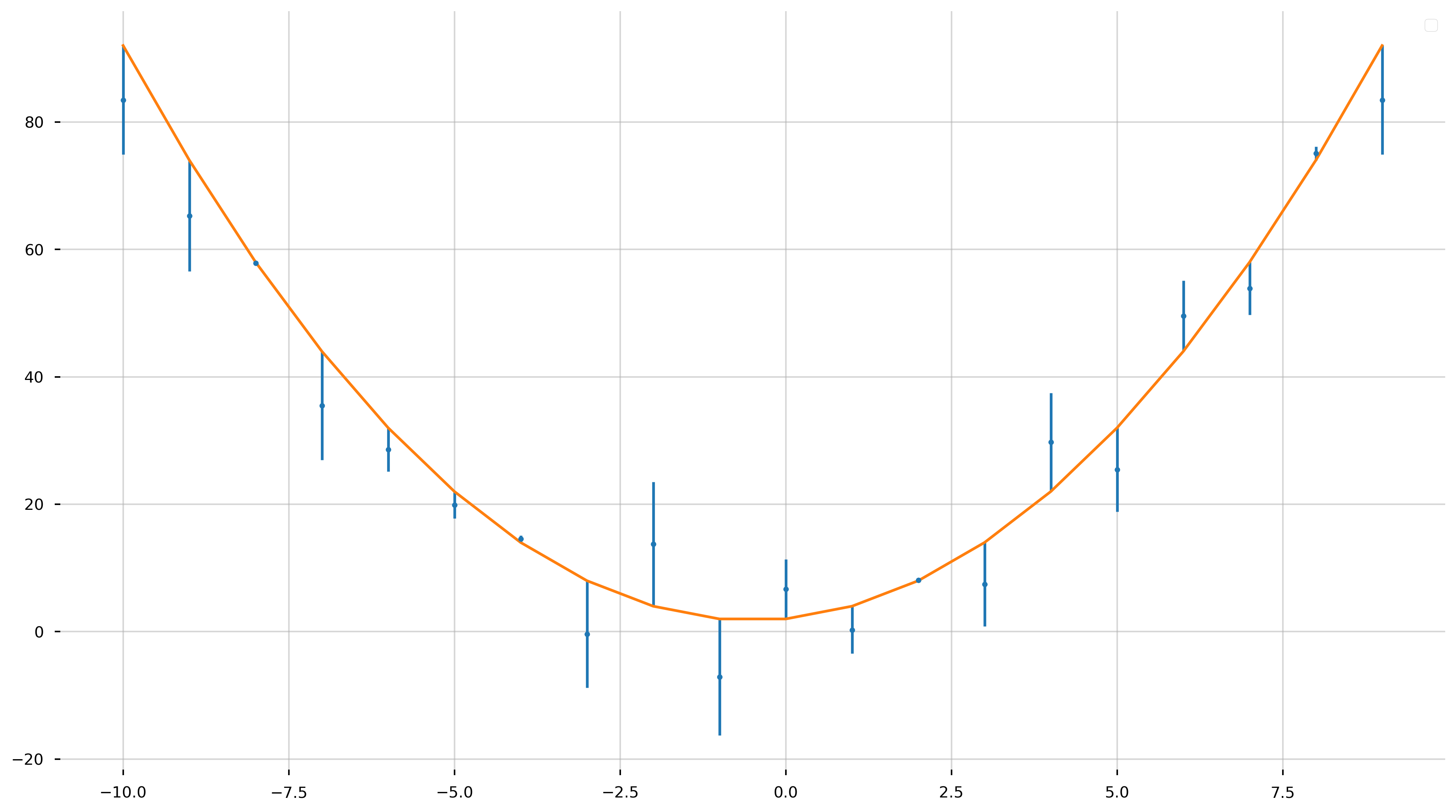
Errorbar Plot
fig = plt.figure(figsize=(16,9))
ax = plt.gca()

x = np.arange(-10, 10, 1)
y = x**2 + x + 2.0
yerr = np.random.uniform(-10, 10, size=len(x)) # fake error

ax.errorbar(x, y+yerr, yerr, fmt='.')
ax.plot(x, y) # over plot the true
Final Exercise
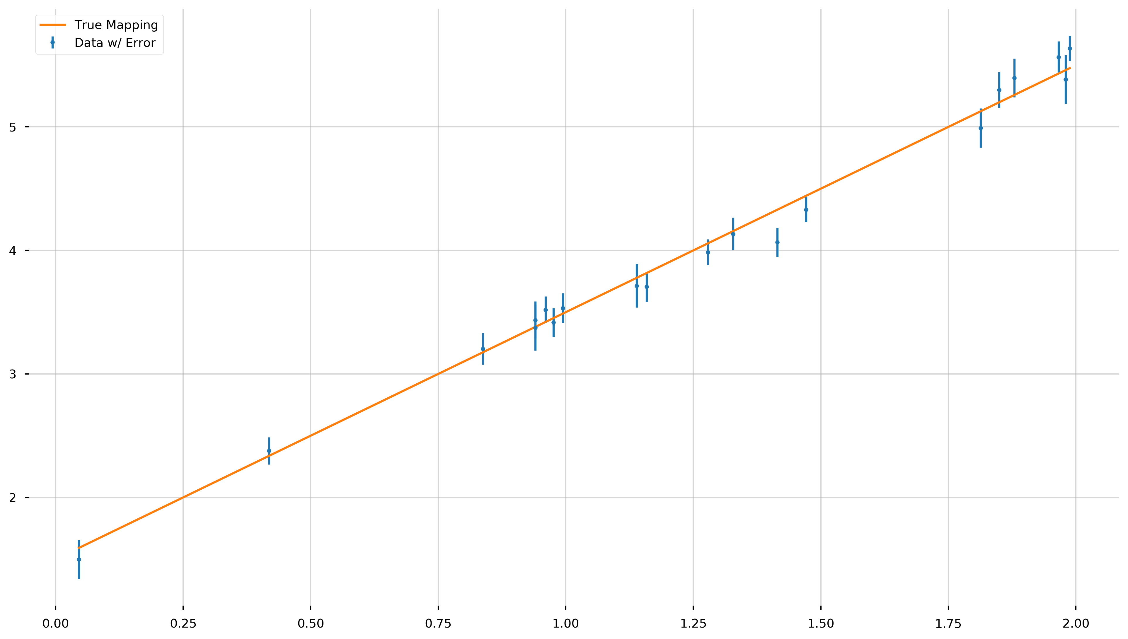
What we will do now is create some fake data generated from a simple model—a line—then we will “scramble” the data by adding some random noise. Next seminar, we will attempt to “recover” the mapping, \(X \to Y\). That is to say, figure out the underlying model by which the data was created.
Let us define a true slope, \(m=2.0\), and a true intercept $b=1.5$.
1) Randomly generate an array of 20 uniformly-distributed x values from the domain (0,2).
2) Sort the values in ascending order.
3) Define a variable, \(y_{true}\), which evalues the following:
\[y_{true} = m\cdot x + b\]4) Define a variable, \(y_{err}\), which is an array of uniformly sampled values between 0.1 and 0.2 of the same size as x.
5) Resample \(y\) data with noise from a normal distribution. That is to say,
\(y \sim \mathcal{N} [\mu = y_{true}, \sigma = y_{err}]\) where \(\mu\) is the mean, and \(\sigma\) is the standard deviation. hint: np.normal()
6) Produce an error bar plot, with x on the x-axis, y on the y-axis, and yerr as error bars.
7) Overplot as a line, the \(y_{true}\) against \(x\).
Final Exercise Solution
# (0)
m = 2.0 #slope
b = 1.5 #intercept

# (1)
x = np.random.uniform(0, 2, 20)

# (2)
x.sort()

# (3)
y_true = m*x + b

# (4)
y_err = np.random.uniform(0.1, 0.2, size=len(x))

# (5)
y = np.random.normal(y_true, y_err)

fig = plt.figure(figsize=(16,9))
ax = plt.gca()

# (6)
ax.errorbar(x, y, y_err, fmt='.', label='Data w/ Error')

# (7)
ax.plot(x, y_true, label='True Mapping')